多变量模式分析:Multivariate pattern analysis (MVPA)
问题:多变量在fMRI的情境下是“多体素”,那么在EEG的情境下代表什么呢?
Kimi:在EEG(脑电图)的情境下,多变量分析通常指的是分析多个电极通道上记录的脑电信号模式。与fMRI中的“多体素”相对应,在EEG中,我们关注的是“多电极”或“多通道”上的信息。这种分析方法可以揭示不同脑区之间在时间和空间上的动态相互作用,以及它们在认知和感知任务中的协调活动
EEG2EEG中用到两种MVPA方法:基于分类的解码和表征相似性解码来分析生成数据与真实数据中的神经表示。基于分类的解码是比较图像之间的解码精度,而表征相似性解码分析脑电数据和模型层之间的相似度。
基于分类的解码:使用线性支持向量机 (SVM) 对每个 10 毫秒时间窗口的单试次水平测试数据上每对图像的神经模式进行分类,时间步长为 10 毫秒。分类器针对每个时间窗口独立训练和测试。为了提高信噪比,我们从相同的图像条件下平均每5次试验。使用一个5 × 4折交叉验证框架。对所有图像对的解码准确率进行平均,并与50%的随机水平进行比较。解码精度越高表明神经模式之间的差异越大。对于真实数据,对每个受试者分别执行解码分析。对于生成数据,对所有72个目标主体数据分别执行解码分析。
表征相似度分析:先前的研究表明,卷积神经网络 (DCNN) 中的层从low-level到high-level捕获视觉信息的神经表示。我们通过计算EEG和DCNN的表征差异矩阵(representational dissimilarity matrices, RDMs)进行比较,比较了人脑和预训练的DCNN之间的200个测试图像的表示。每个 RDM 的形状为 200 × 200。对于 EEG RDM,我们将两个图像条件之间的解码精度(这里的解码精度是指什么呢?)作为差异指数,为每个时间窗口和每个受试者构建 EEG RDM。我们基于真实数据获得了 9 组 20 个 RDM,基于生成的数据获得了 72 组 20 个 RDM(每 10 毫秒作为计算 RDM 的时间窗口)。对于DCNN RDM,我们将所有200张图像输入到在ImageNet上预训练的AlexNet中,并从每一层提取特征。然后我们计算一个负的(减去)对应于任意两个图像的激活向量之间的 Pearson 相关系数作为每一层的 RDM 中的差异指数。此外,我们还直接基于原始图像计算了low-level RDM。因此,我们获得了8个RDM,对应于AlexNet中的8个层和1个低级RDM。为了比较这些表示,我们计算了Spearman相关系数作为EEG RDM和DCNN RDM之间的相似性。解码和RSA分析都是基于NeuroRA工具箱实现的。
问题:为什么计算RDM中的差异指数时用Pearson 相关系数,而计算RDM之间的相似性时用Spearman相关系数呢?
https://www.genedenovo.com/news/293.html
适用范围与计算方法选择
Spearman 和Pearson相关系数在算法上完全相同. 只是Pearson相关系数是用原来的数值计算积差相关系数, 而Spearman是用原来数值的秩次计算积差相关系数。
1、Pearson相关系数适用条件为两个变量间有线性关系、变量是连续变量、变量均符合正态分布。
2、若上述有条件不满足则考虑用Spearman相关系数
3、对于同一量纲数据建议Pearson,例如mRNA表达量数据,计算不同
mRNA表达量的相关系数;对于不同量纲数据,可考虑Spearman相关系数,例如mRNA表达量与某表型数据(株高、产果量、次生化合物含量等)
代码精读
Decoding_RSA.py
这个文件里的代码应该是关于Classification-based decoding的,让我们来看看:
import numpy as np
from neurora.rdm_cal import eegRDM_bydecoding
from neurora.rsa_plot import plot_tbyt_decoding_acc, plot_tbytsim_withstats, plot_rdm
from neurora.corr_cal_by_rdm import rdms_corr
from neurora.rdm_corr import rdm_correlation_spearman
import matplotlib.pyplot as plt
from scipy.stats import ttest_1samp


for i in range(10):
    if i != 8:
        real = np.load('/home/user/lanyinyu/EEG2EEG/eeg_data/test/st_sub' + str(i + 1).zfill(2) + '.npy')
        real = np.transpose(real, (1, 2, 0, 3))
        # data: [nconditions * ntrials * nchannels * nts]

        real = np.reshape(real, [200, 1, 80, 17, 200])

        real_eegRDMs = eegRDM_bydecoding(real, sub_opt=1, time_win=10, time_step=10, nfolds=4, nrepeats=5)[0]

        np.save('/home/user/lanyinyu/EEG2EEG/Analysis_results/decoding_RSA/realeegRDMs_Sub' + str(i+1) + '.npy', real_eegRDMs)


for i in range(10):
    if i != 8:
        fake_eegRDMs = np.zeros([8, 20, 200, 200])
        index = 0
        for j in range(10):
            if j != 8 and j != i:
                fake = fake = np.load('/home/user/lanyinyu/EEG2EEG/generated_fullmodel/st_Sub' + str(i + 1) + 'ToSub' + str(j + 1) + '_final.npy')
                fake = np.transpose(fake, (1, 2, 0, 3))
                # data: [nconditions * ntrials * nchannels * nts]

                fake = np.reshape(fake, [200, 1, 80, 17, 200])

                fake_eegRDMs[index] = eegRDM_bydecoding(fake, sub_opt=1, time_win=10, time_step=10, nfolds=4, nrepeats=5)[0]

                index += 1

        np.save('/home/user/lanyinyu/EEG2EEG/Analysis_results/decoding_RSA/fakeeegRDMs_fromSub' + str(i+1) + '.npy', fake_eegRDMs)
这里调用了neurora中的eegRDM_bydecoding输入EEG生成RDM,继续看看eegRDM_bydecoding源码:
' a function for calculating the RDM(s) using classification-based neural decoding based on EEG/MEG/fNIRS & other EEG-like data '

def eegRDM_bydecoding(EEG_data, sub_opt=1, time_win=5, time_step=5, navg=5, time_opt="average", nfolds=5, nrepeats=2,normalization=False):

    """
    Calculate the Representational Dissimilarity Matrix(Matrices) - RDM(s) using classification-based neural decoding
    based on EEG-like data

    Parameters
    ----------
    EEG_data : array
        The EEG/MEG/fNIRS data.
        The shape of EEGdata must be [n_cons, n_subs, n_trials, n_chls, n_ts].
        n_cons, n_subs, n_trials, n_chls & n_ts represent the number of conidtions, the number of subjects, the number
        of trials, the number of channels & the number of time-points, respectively.
    sub_opt: int 0 or 1. Default is 1.
        Return the subject-result or average-result.
        If sub_opt=0, return the average result.
        If sub_opt=1, return the results of each subject.
    time_win : int. Default is 5.
        Set a time-window for calculating the RDM for different time-points.
        Only when time_opt=1, time_win works.
        If time_win=5, that means each calculation process based on 5 time-points.
    time_step : int. Default is 5.
        The time step size for each time of calculating.
        Only when time_opt=1, time_step works.
    navg : int. Default is 5.
        The number of trials used to average.
    time_opt : string "average" or "features". Default is "average".
        Average the time-points or regard the time points as features for classification
        If time_opt="average", the time-points in a certain time-window will be averaged.
        If time_opt="features", the time-points in a certain time-window will be used as features for classification.
    nfolds : int. Default is 5.
        The number of folds.
        k should be at least 2.
    nrepeats : int. Default is 2.
        The times for iteration.
    normalization : boolean True or False. Default is False.
        Normalize the data or not.

    Returns
    -------
    RDM(s) : array
        The EEG/MEG/fNIR/other EEG-like RDM.
        If sub_opt=0, return int((n_ts-time_win)/time_step)+1 RDMs.
            The shape is [int((n_ts-time_win)/time_step)+1, n_cons, n_cons].
        If sub_opt=1, return n_subs*int((n_ts-time_win)/time_step)+1 RDM.
            The shape is [n_subs, int((n_ts-time_win)/time_step)+1, n_cons, n_cons].

    Notes
    -----
    Sometimes, the numbers of trials under different conditions are not same. In NeuroRA, we recommend users to sample
    randomly from the trials under each conditions to keep the numbers of trials under different conditions same, and
    you can iterate multiple times.
    """

    if len(np.shape(EEG_data)) != 5:

        print("The shape of input for eegRDM() function must be [n_cons, n_subs, n_trials, n_chls, n_ts].\n")

        return "Invalid input!"

    # get the number of conditions, subjects, trials, channels and time points
    cons, subs, trials, chls, ts = np.shape(EEG_data)

    ts = int((ts - time_win) / time_step) + 1

    rdms = np.zeros([subs, ts, cons, cons])

    for con1 in range(cons):
        for con2 in range(cons):

            if con1 > con2:

                data = np.concatenate((EEG_data[con1], EEG_data[con2]), axis=1)
                labels = np.zeros([subs, 2*trials])
                labels[:, trials:] = 1
                rdms[:, :, con1, con2] = tbyt_decoding_kfold(data, labels, n=2, navg=navg, time_opt=time_opt,time_win=time_win, time_step=time_step, nfolds=nfolds,nrepeats=nrepeats, normalization=normalization,pca=False, smooth=True)
                rdms[:, :, con2, con1] = rdms[:, :, con1, con2]

    if sub_opt == 0:

        return np.average(rdms, axis=0)

    else:

        return rdms
这是一个对EEG形式脑电信号数据进行基于分类的神经解码计算RDM的函数。输入包括9个参数,EEG_data是输入的脑电数据,形式是[n_cons, n_subs, n_trials, n_chls, n_ts]的数组,n_cons、n_subs、n_trials、n_chls 和 n_ts 分别代表条件数、受试者数、试验数、通道数和时间点数。sub_opt是整数0或者1,默认为1,0表示返回平均结果,1表示返回所有个体的结果。time_win是时间窗口的大小。time_step是时间步长大小。navg是平均试次的大小。time_opt :对时间点取平均值或将时间点作为分类的特征。如果time_opt="average",则对某个时间窗口内的时间点取平均值。如果time_opt="features",则将某个时间窗口内的时间点作为分类的特征。nfolds是折数。nrepeats是迭代次数。normalization是归一化选项。再来看下输出的RDM,形式为array数组,如果sub_opt=0, 返回int((n_ts-time_win)/time_step)+1(总时间步数)个RDM,形状为[int((n_ts-time_win)/time_step)+1, n_cons, n_cons],如果sub_opt=1,则前面多一个受试者数的维度。有时不同条件下的试验次数并不相同。在 NeuroRA 中,建议用户从各个条件下的试验中随机抽取样本,以保持不同条件下的试验次数相同。
代码逻辑:两两计算不同条件下的RDM,会给两种条件的数据拼接起来,打上0和1的标签,这里调用了tbyt_decoding_kfold函数计算RDM,再继续简单看下该函数:
def tbyt_decoding_kfold(data, labels, n=2, navg=5, time_opt="average", time_win=5, time_step=5, nfolds=5, nrepeats=2,normalization=False, pca=False, pca_components=0.95, smooth=True):

    """
    Conduct time-by-time decoding for EEG-like data (cross validation)

    Parameters
    ----------
    data : array
        The neural data.
        The shape of data must be [n_subs, n_trials, n_chls, n_ts]. n_subs, n_trials, n_chls and n_ts represent the
        number of subjects, the number of trails, the number of channels and the number of time-points.
    labels : array
        The labels of each trial.
        The shape of labels must be [n_subs, n_trials]. n_subs and n_trials represent the number of subjects and the
        number of trials.
    n : int. Default is 2.
        The number of categories for classification.
    navg : int. Default is 5.
        The number of trials used to average.
    time_opt : string "average" or "features". Default is "average".
        Average the time-points or regard the time points as features for classification
        If time_opt="average", the time-points in a certain time-window will be averaged.
        If time_opt="features", the time-points in a certain time-window will be used as features for classification.
    time_win : int. Default is 5.
        Set a time-window for decoding for different time-points.
        If time_win=5, that means each decoding process based on 5 time-points.
    time_step : int. Default is 5.
        The time step size for each time of decoding.
    nfolds : int. Default is 5.
        The number of folds.
        k should be at least 2.
    nrepeats : int. Default is 2.
        The times for iteration.
    normalization : boolean True or False. Default is False.
        Normalize the data or not.
    pca : boolean True or False. Default is False.
        Apply principal component analysis (PCA).
    pca_components : int or float. Default is 0.95.
        Number of components for PCA to keep. If 0<pca_components<1, select the numbder of components such that the
        amount of variance that needs to be explained is greater than the percentage specified by pca_components.
    smooth : boolean True or False, or int. Default is True.
        Smooth the decoding result or not.
        If smooth = True, the default smoothing step is 5. If smooth = n (type of n: int), the smoothing step is n.

    Returns
    -------
    accuracies : array
        The time-by-time decoding accuracies.
        The shape of accuracies is [n_subs, int((n_ts-time_win)/time_step)+1].
    """

    if np.shape(data)[0] != np.shape(labels)[0]:

        print("\nThe number of subjects of data doesn't match the number of subjects of labels.\n")

        return "Invalid input!"

    if np.shape(data)[1] != np.shape(labels)[1]:

        print("\nThe number of epochs doesn't match the number of labels.\n")

        return "Invalid input!"

    nsubs, ntrials, nchls, nts = np.shape(data)

    ncategories = np.zeros([nsubs], dtype=int)

    labels = np.array(labels)

    for sub in range(nsubs):

        sublabels_set = set(labels[sub].tolist())
        ncategories[sub] = len(sublabels_set)

    if len(set(ncategories.tolist())) != 1:

        print("\nInvalid labels!\n")

        return "Invalid input!"

    if n != ncategories[0]:

        print("\nThe number of categories for decoding doesn't match ncategories (" + str(ncategories) + ")!\n")

        return "Invalid input!"

    categories = list(sublabels_set)

    newnts = int((nts-time_win)/time_step)+1

    if time_opt == "average":

        avgt_data = np.zeros([nsubs, ntrials, nchls, newnts])

        for t in range(newnts):
            avgt_data[:, :, :, t] = np.average(data[:, :, :, t * time_step:t * time_step + time_win], axis=3)

        acc = np.zeros([nsubs, newnts])

        total = nsubs * nrepeats * newnts * nfolds

        for sub in range(nsubs):

            ns = np.zeros([n], dtype=int)

            for i in range(ntrials):
                for j in range(n):
                    if labels[sub, i] == categories[j]:
                        ns[j] = ns[j] + 1

            minn = int(np.min(ns) / navg)

            subacc = np.zeros([nrepeats, newnts, nfolds])

            for i in range(nrepeats):

                datai = np.zeros([n, minn * navg, nchls, newnts])
                labelsi = np.zeros([n, minn], dtype=int)

                for j in range(n):
                    labelsi[j] = j

                randomindex = np.random.permutation(np.array(range(ntrials)))

                m = np.zeros([n], dtype=int)

                for j in range(ntrials):
                    for k in range(n):

                        if labels[sub, randomindex[j]] == categories[k] and m[k] < minn * navg:
                            datai[k, m[k]] = avgt_data[sub, randomindex[j]]
                            m[k] = m[k] + 1

                avg_datai = np.zeros([n, minn, nchls, newnts])

                for j in range(minn):
                    avg_datai[:, j] = np.average(datai[:, j * navg:j * navg + navg], axis=1)

                x = np.reshape(avg_datai, [n * minn, nchls, newnts])
                y = np.reshape(labelsi, [n * minn])

                for t in range(newnts):

                    state = np.random.randint(0, 100)
                    kf = StratifiedKFold(n_splits=nfolds, shuffle=True, random_state=state)
                    xt = x[:, :, t]

                    fold_index = 0
                    for train_index, test_index in kf.split(xt, y):

                        x_train = xt[train_index]
                        x_test = xt[test_index]

                        if normalization is True:
                            scaler = StandardScaler()
                            x_train = scaler.fit_transform(x_train)
                            x_test = scaler.transform(x_test)

                        if pca is True:

                            Pca = PCA(n_components=pca_components)
                            x_train = Pca.fit_transform(x_train)
                            x_test = Pca.transform(x_test)

                        svm = SVC(kernel='linear', tol=1e-4, probability=False)
                        svm.fit(x_train, y[train_index])
                        subacc[i, t, fold_index] = svm.score(x_test, y[test_index])

                        percent = (sub * nrepeats * newnts * nfolds + i * newnts * nfolds + t * nfolds + fold_index + 1) / total * 100
                        show_progressbar("Calculating", percent)

                        if sub == (nsubs - 1) and i == (nrepeats - 1) and t == (newnts - 1) and fold_index == (
                                nfolds - 1):
                            print("\nDecoding finished!\n")

                        fold_index = fold_index + 1

            acc[sub] = np.average(subacc, axis=(0, 2))

    if time_opt == "features":

        avgt_data = np.zeros([nsubs, ntrials, nchls, time_win, newnts])

        for t in range(newnts):
            avgt_data[:, :, :, :, t] = data[:, :, :, t * time_step:t * time_step + time_win]

        avgt_data = np.reshape(avgt_data, [nsubs, ntrials, nchls*time_win, newnts])

        acc = np.zeros([nsubs, newnts])

        total = nsubs * nrepeats * newnts * nfolds

        for sub in range(nsubs):

            ns = np.zeros([n], dtype=int)

            for i in range(ntrials):
                for j in range(n):
                    if labels[sub, i] == categories[j]:
                        ns[j] = ns[j] + 1

            minn = int(np.min(ns) / navg)

            subacc = np.zeros([nrepeats, newnts, nfolds])

            for i in range(nrepeats):

                datai = np.zeros([n, minn * navg, nchls * time_win, newnts])
                labelsi = np.zeros([n, minn], dtype=int)

                for j in range(n):
                    labelsi[j] = j

                randomindex = np.random.permutation(np.array(range(ntrials)))

                m = np.zeros([n], dtype=int)

                for j in range(ntrials):
                    for k in range(n):

                        if labels[sub, randomindex[j]] == categories[k] and m[k] < minn * navg:
                            datai[k, m[k]] = avgt_data[sub, randomindex[j]]
                            m[k] = m[k] + 1

                avg_datai = np.zeros([n, minn, nchls * time_win, newnts])

                for j in range(minn):
                    avg_datai[:, j] = np.average(datai[:, j * navg:j * navg + navg], axis=1)

                x = np.reshape(avg_datai, [n * minn, nchls * time_win, newnts])
                y = np.reshape(labelsi, [n * minn])

                for t in range(newnts):

                    state = np.random.randint(0, 100)
                    kf = StratifiedKFold(n_splits=nfolds, shuffle=True, random_state=state)
                    xt = x[:, :, t]

                    fold_index = 0
                    for train_index, test_index in kf.split(xt, y):

                        x_train = xt[train_index]
                        x_test = xt[test_index]

                        if normalization is True:
                            scaler = StandardScaler()
                            x_train = scaler.fit_transform(x_train)
                            x_test = scaler.transform(x_test)

                        if pca is True:

                            Pca = PCA(n_components=pca_components)
                            x_train = Pca.fit_transform(x_train)
                            x_test = Pca.transform(x_test)

                        svm = SVC(kernel='linear', tol=1e-4, probability=False)
                        svm.fit(x_train, y[train_index])
                        subacc[i, t, fold_index] = svm.score(x_test, y[test_index])

                        percent = (sub * nrepeats * newnts * nfolds + i * newnts * nfolds + t * nfolds + fold_index + 1) / total * 100
                        show_progressbar("Calculating", percent)

                        if sub == (nsubs - 1) and i == (nrepeats - 1) and t == (newnts - 1) and fold_index == (
                                nfolds - 1):
                            print("\nDecoding finished!\n")

                        fold_index = fold_index + 1

            acc[sub] = np.average(subacc, axis=(0, 2))

    if smooth is False:

        return acc

    if smooth is True:

        smooth_acc = smooth_1d(acc)

        return smooth_acc

    else:

        smooth_acc = smooth_1d(acc, n=smooth)

        return smooth_acc
该函数的作用是对EEG形式数据进行逐时解码(交叉验证),除了继承的参数以外,多了pca,pca_components,smooth三个参数,PCA表示是否应用主成分分析,pca_components默认值为0.95。PCA 保留的成分数。如果 0<pca_components<1,则选择成分数,使得需要解释的方差量大于 pca_components 指定的百分比。smooth表示是否平滑解码的结果,根据时间点前后n个值进行平均。代码调用了sklearn中的算法,使用SVM进行分类。
OK,再回到Decoding_RSA.py文件,看下一段代码:
# real - acc
realaccs = np.zeros([9, 20])
index1 = 0
for i1 in range(10):
    if i1 != 8:
        realRDMs = np.load('Analysis_results/decoding_RSA/realeegRDMs_Sub' + str(i1+1) + '.npy')
        for j in range(200):
            for k in range(200):
                if j > k:
                    realaccs[index1] += realRDMs[:, j, k]
        index1 += 1
realaccs = realaccs/19900

plot_tbyt_decoding_acc(realaccs, start_time=0, end_time=0.2, time_interval=0.01, xlim=[0, 0.2], ylim=[0.4, 0.9], cbpt=False, avgshow=True)


# fake - acc
fakeaccs = np.zeros([72, 20])
index1 = 0
for i1 in range(10):
    if i1 != 8:
        fakeRDMs = np.load('Analysis_results/decoding_RSA/fakeeegRDMs_fromSub' + str(i1+1) + '.npy')
        for i2 in range(8):
            for j in range(200):
                for k in range(200):
                    if j > k:
                        fakeaccs[index1*8+i2] += fakeRDMs[i2, :, j, k]
        index1 += 1
fakeaccs = fakeaccs/19900

plot_tbyt_decoding_acc(fakeaccs, start_time=0, end_time=0.2, time_interval=0.01, xlim=[0, 0.2], ylim=[0.4, 0.9], cbpt=False,
                       avgshow=True)
这里画的是真实数据(上)和生成数据(下)随时间解码准确率的图:
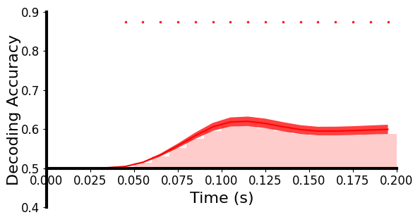
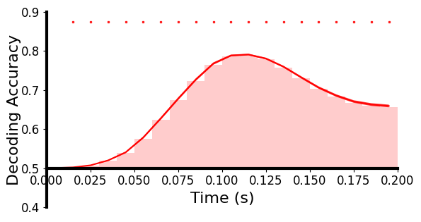
我们注意到这幅图,横坐标是时间,纵坐标是解码精度,柱形图表示时间段的精度,柱形图有近似曲线和曲线区间,最上面还有小点看起来是表示显著性的,看下plot_tbyt_decoding_acc函数:
def plot_tbyt_decoding_acc(acc, start_time=0, end_time=1, time_interval=0.01, chance=0.5, p=0.05, cbpt=True,
                           clusterp=0.05, stats_time=[0, 1], color='r', xlim=[0, 1], ylim=[0.4, 0.8],
                           xlabel='Time (s)', ylabel='Decoding Accuracy', figsize=[6.4, 3.6], x0=0, labelpad=0,
                           ticksize=12, fontsize=16, markersize=2, title=None, title_fontsize=16, avgshow=False):
acc是准确率,形状为[n_subs, n_ts],start_time默认是0,end_time默认是1,time_interval是两个样本间的时间间隔,chance是随机水平,p是p值阈值,cbpt是是否进行基于聚类的排列测试,clusterp是聚类定义p值的阈值,stats_time是统计分析的时间段(跟start_time、end_time是不是重叠了?),color是matplotlib画的曲线颜色,xlim和ylim是x轴和y轴的视图区间限制,xlabel、ylabel是轴标签,figsize是表格大小,x0是y轴位置,labelpad是y轴标签离y轴的距离,ticksize是刻度大小,fontsize是字体大小,markersize是显著性标记的大小,title是图片标题,title_fontsize是标题字体大小,avgshow表示是否展示平均解码精度。
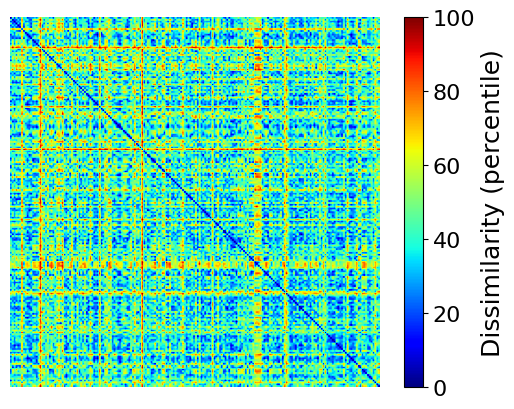
使用neurora.rsa_plot里的plot_rdm可视化一个 200 × 200 的RDM矩阵看看:
RSA.py
这个文件里的代码应该是关于Representational similarity analysis的,让我们来看看: